Generating the Variables

I started with the authors. html_node(".author") selects all the objects within the author class from reviews. The output is a vector of a length of the reviews. Each element in the list is a node with the class author. For example: <a href="https://old.reddit.com/user/Hendrix194" class="author may-blank id-t2_n4hdv">Hendrix194</a>. This would be useless unless you call other functions from rvest, i.e. html_text(). It extracts the selector content that is, in this case, the author’s name: Hendrix194!

Author

author <- reviews %>%
  html_node(".author") %>%
  html_text()%>%
  str_trim() 

author <- as.factor(author)

After obtaining and examining the value author, I found several [deleted] values. Initially, I thought these authors and their comments were deleted. However, for whatever reason, the comments were still visible. Therefore, I decided to not dispose them. Finally, I stored the vector as a factor because each author is an individual entity.

Comment

Naturally, each comment is the most important variable for my analysis. The approach was identical to scraping author. Once again, the function selects all the objects with the class. In addition to solely extracting the selector content by html_text(), I specified an additional argument trim = TRUE. trim eliminates any space character (which is invisible to human eye) before and after a string. Additionally, I dispose of newline separators \n by calling the gsub() function and specifying the pattern as the function’s argument.

comment <- reviews %>%
  html_node(".md") %>%
  html_text(trim = TRUE ) %>%
  gsub("\n","",.)

After I extracted the content of .score, I ended up with a string vector where each value was composed of two words. Additionally, the first word was supposed to be numeric, e.g. "3 points". To get it, I simply supplied 1; i.e. specified the position of my word of interest, as the argument inside stringr::word() and piped the result into as.integer().

# library(stringr)

likes <- reviews %>%
  html_node(".score") %>%
  html_text() %>%
  word(1) %>%
  as.integer() 

Initially, I thought I would only be able to scrape the time variable as it is displayed on Reddit, e.g. "3 months ago". Fortunately, such format is the output of java, which together with the HTML and CSS, makes any website’s content readable to a human. Note, that I also did not extract selector’s content as I did with the previous variables.

Finally, I formatted time with the base striptime() function and transformed it by ymd_hms() into POSIXct. Such formatting may have major benefits when analyzing sentiments in units of minutes, seconds but also at lower frequencies!

# lubridate
date <- reviews %>%
  html_node("time")%>%
  html_attr("title")%>%
  strptime(format = "%a %b %d %H:%M:%S %Y",tz = "UTC")%>%
  ymd_hms()

Data Frames

I ended up with 4 vectors. Firstly, I merged all of them into one data frame dataset. I also called filter and mutate to simultaneously clean the data a little bit and create id - a unique value to every comment. dataset is my entry level data frame for two additional tidy datasets. Additionally, it is easy to search for any id and examine the associated comment.

# Data frame from vectors
dataset <- data.frame(author, likes, comment, date, stringsAsFactors = FALSE) %>%
  filter(!is.na(author))%>%
  # Filtering comments of few words
  filter(str_count(comment)>=5) %>%
  # creating ID for each comment so I can refer to it later
  mutate(id = row_number())

Secondly, it was necessary to clean dataset$comment. Specifically, any stop words, single and meaningless characters, and numbers that are redundant for the majority of text analysis. My goal was to create a new tidy data frame where each observation would be a single word from the comment it appears in. I achieved that through tidytext::unnest_tokens(), tidytext::stop_words, dplyr::anti_join(). unnest_token() takes three arguments: i.) dataset, ii.) new variable (word), and iii.) name of a string column (comment). The output is the tidy data frame where number of rows per entity (comment or id) is equal to number of words in comment. It is also worthy of mention that the function sets all the letters to lower case by default. I also called anti_join() three times to filter: i.) stop words (stop_words is a vector of the stop words from tidytext), ii.) URL links (url_words), iii.) and numeric strings. Note that the argument in anti_join() must not be a vector! Finally, I filtered any words of lower length or equal to 3 characters.

#tidytext
url_words <- tibble(
  word = c("https","http")) #filternig weblinks

tidy_data <- dataset %>% unnest_tokens(word, comment) %>% anti_join(stop_words, by="word") %>%  anti_join(url_words, by="word") %>% 
# filtering "numeric" words  
anti_join(tibble(word = as.character (c(1:10000000))), by="word") %>%
# stop word already filter but there were still redundent words, e.g. nchar(word) < 3
  filter(nchar(word)>=3) 

rm(url_words)

Lastly, I created data_sentiment data frame from tidy_data. I achieved that by filtering and joining the data from nrc lexicon. I had chosen nrc because it contains a variety of emotions associated with the word. I also created author_total, i.e. how many words in total has each author posted to the forum. inner_join(get_sentiments("nrc"), by="word") joins nrc lexicon with sentiments to tidy_data. Note that inner_join() filters out any words out of the intersection of any two data sets.

data_sentiment <- tidy_data %>% 
    # Group by author
    group_by(author) %>% 
    # Define a new column author_total; i.e. how many words an author has posted
    mutate(author_total=n()) %>%
    ungroup() %>%
    # Implement sentiment analysis with the NRC lexicon
    inner_join(get_sentiments("nrc"), by="word")

These steps above summarize my preprocessing and data cleaning strategies. Having three different data sets, there was nothing else impeding the analysis. From this step, it was easy to explore and analyze the data more precisely.

Exploratory Data Analysis (EDA)

Collecting any time varying variable, one should always know the time span.

range(dataset$date) #time span

## [1] "2018-10-17 04:17:53 UTC" "2019-03-10 04:45:13 UTC"

range(dataset$date)[2]-range(dataset$date)[1]

## Time difference of 144.019 days

Interesting! The very first comment on the forum was posted on the day when legalization happened, i.e. 2018-10-17. On the other hand, the last comment was submitted (in time of writing this post) in March 2019. This tells us the discussion has been alive for 145 days, i.e. almost 5 months. Initially, I thought that the time frame would be sufficient for interesting observations and conclusions. However, the frequency of new comments matters as well. Is there a representative number of submitted comments for each month? One way to answer the question would be a visual examination.

The following plot displays the count of new comments in time.

dataset %>% select(date,comment) %>% 
  mutate(date = round_date(date, "1 day"))  %>% group_by(date) %>% mutate(n_comments = n()) %>% 
  # filter(date < ymd("2018-10-25")) %>%
  # Had to round  up the date object into "week" units, otherwise grouping a mutating would not work   (too narrow interval)

  ggplot(aes(date,n_comments)) +
  geom_line(linetype = 1)+
  ggtitle("Number of Comments in Time")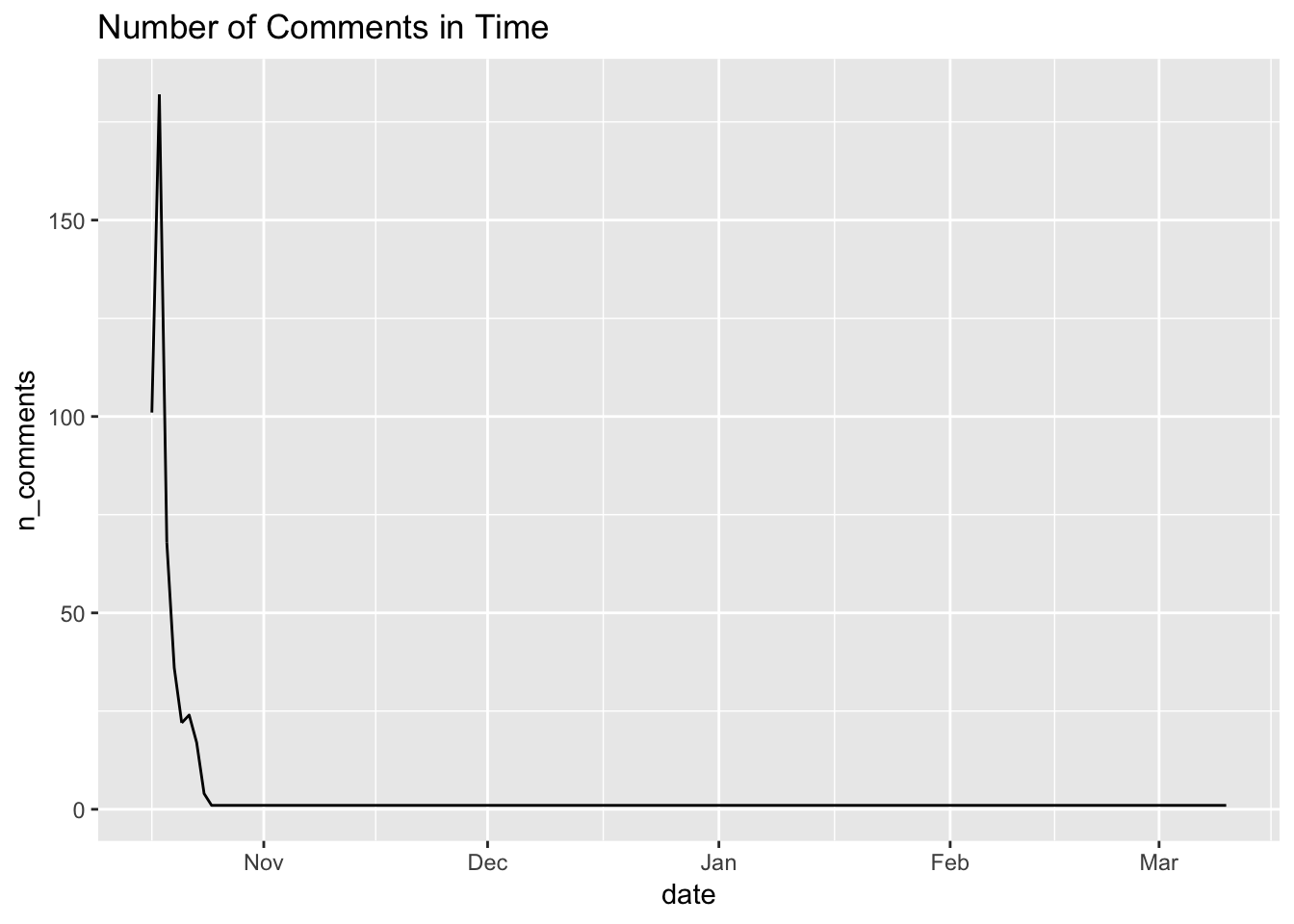

Unfortunately, the discussion was truly “alive” only a few weeks after October 17th. After the end of October 2018, new comments per day or even month were marginal.

Even though I could not answer my initial questions in the full extent, I could focus on the cannabis consumers’ initial attitude. So how many comments were posted there?

nrow(dataset) # n comments

## [1] 460

Besides the number of comments, and the frequency of new ones, the total of contributors to the discussion should be represented as well.

nlevels(dataset$author) #n levels

## [1] 166

Relative to the total number of comments, I maintain that enough authors have contributed into the discussion.

Text Analysis

Did you already examine this post’s cover picture? It is the word cloud from wordcloud2 package and it displays the most frequent words in the discussion. By default, words with the highest frequency are centered in the middle of the plot. I like word clouds because they are great tools for very first inspection of text data. You can easily infer the subject being discussed.

# library(wordcloud2)

tidy_data %>% select(word) %>% count(word,sort=T) %>%
wordcloud2(backgroundColor = "black", color = "green")

While words like cannabis, legal, weed, etc. would be expected to appear in the discussion, there are other frequent words which may arouse your interest. For example, there are a lot of words associated with online shopping. Among them, ocs (Ontario Cannabis Store), shipping, buy, visa, credit, debit, and card appear most frequently. Such observations suggest that a substantial number of comments in the discussion is about the cannabis business.

Let’s examine some of the comments with those - cannabis business related - words!

tidy_data %>%
  filter(!is.na(likes),word %in% c("ocs", "shipping", "credit", "store", "visa", "debit","buy"))%>%
  group_by(id)%>%
  summarize(n=n())%>%
  arrange(desc(n))%>%
  head(5)

## # A tibble: 5 x 2
##      id     n
##   <int> <int>
## 1   457     4
## 2   147     3
## 3   163     3
## 4   211     3
## 5   450     3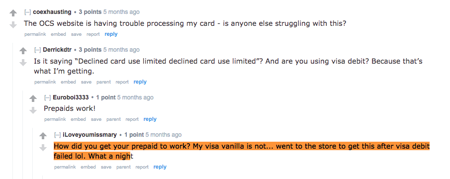

These comments confirm my hypothesis that those words are closely related to the cannabis business. In addition, the author of these comments are concerned about their privacy while making a purchase. It seems like, they are not certain about the privacy involved in buying cannabis with their credit cards.

Who were the most frequent contributors to the discussion? In addition to a “tibble”, as the output of dplyr functions, ggplot2 allows another visual inspection. The following bar plot exhibits the count of comments that the five most frequent contributors to this discussion have posted. However, [deleted] is rather for every unknown author than a specific one.

dataset %>%
  group_by(author) %>%
  summarise(Comments=n())%>%
  arrange(desc(Comments))%>%
  mutate(author = reorder(author, Comments)) %>%
  head(5) %>%
  
  ggplot(aes(author,Comments))+
  geom_col(show.legend = F)+
  coord_flip()+
  geom_text(aes(label = Comments))+
  ggtitle("The Most Frequently Contributing Authors")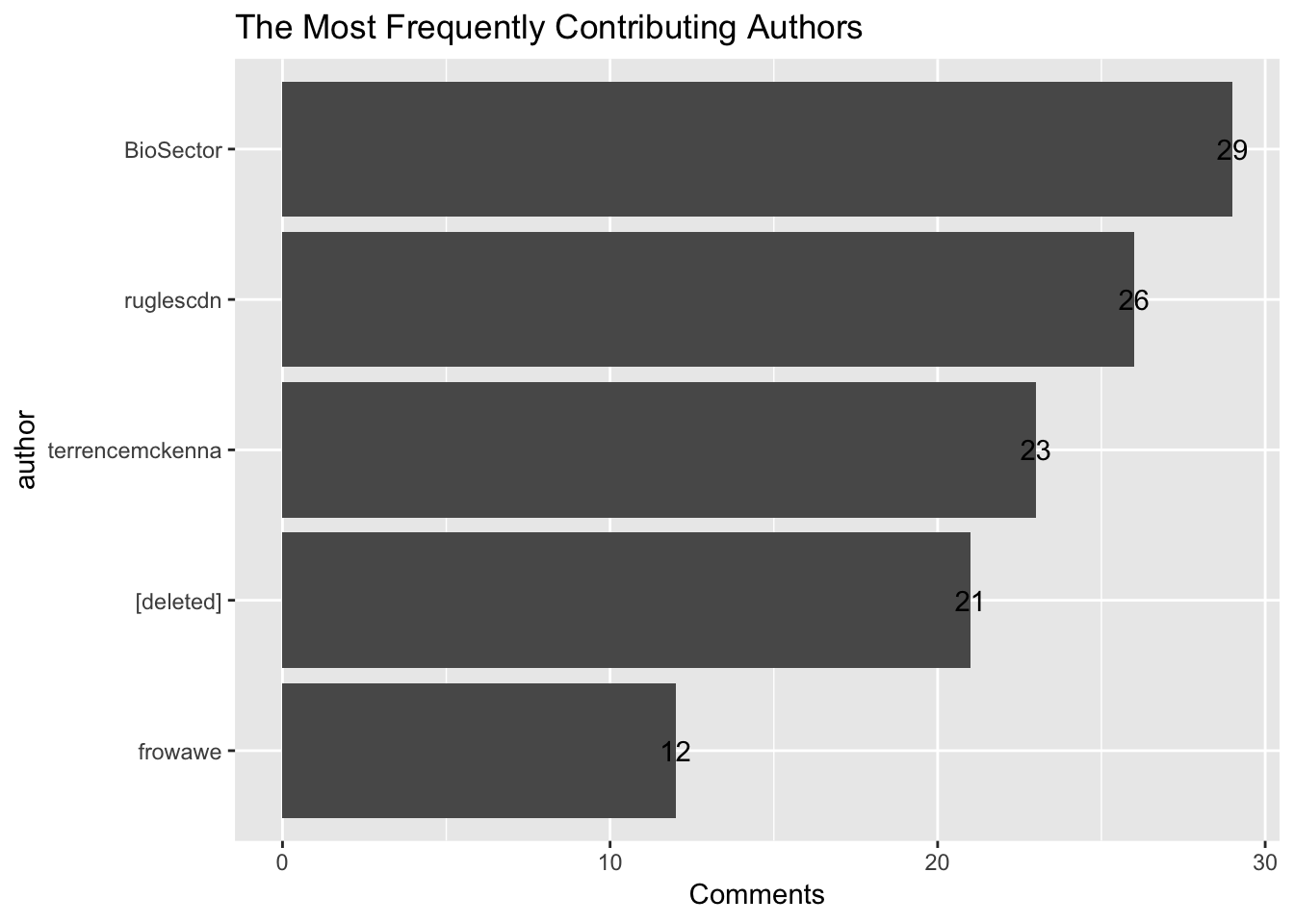

Because I was assuming these contributors have a substantial impact on positive and negative sentiments, I have decided to focus on the words they posted.

The plot below outlines the specific and most frequently used words by their authors. Bear in mind these words come from nrc lexicon. Therefore, the words that were not contained in the lexicon were filtered out. However, the remaining words create the sentiments.

data_sentiment %>%
    # Count by word and author
    count(word,author) %>%
    # Group by author
    group_by(author) %>%
    # Take the top 10 words for each author
    top_n(10) %>%
    ungroup() %>%
    mutate(word = reorder(paste(word, author, sep = "__"), n)) %>%
    filter(author %in% c("BioSector", "ruglescdn",  "terrencemckenna", "frowawe" )) %>%
    # Set up the plot with aes()
    ggplot(aes(word,n)) +
    geom_col(show.legend = FALSE) +
    scale_x_discrete(labels = function(x) gsub("__.+$", "", x)) +
    facet_wrap(~ author, nrow = 2, scales = "free") +
    coord_flip()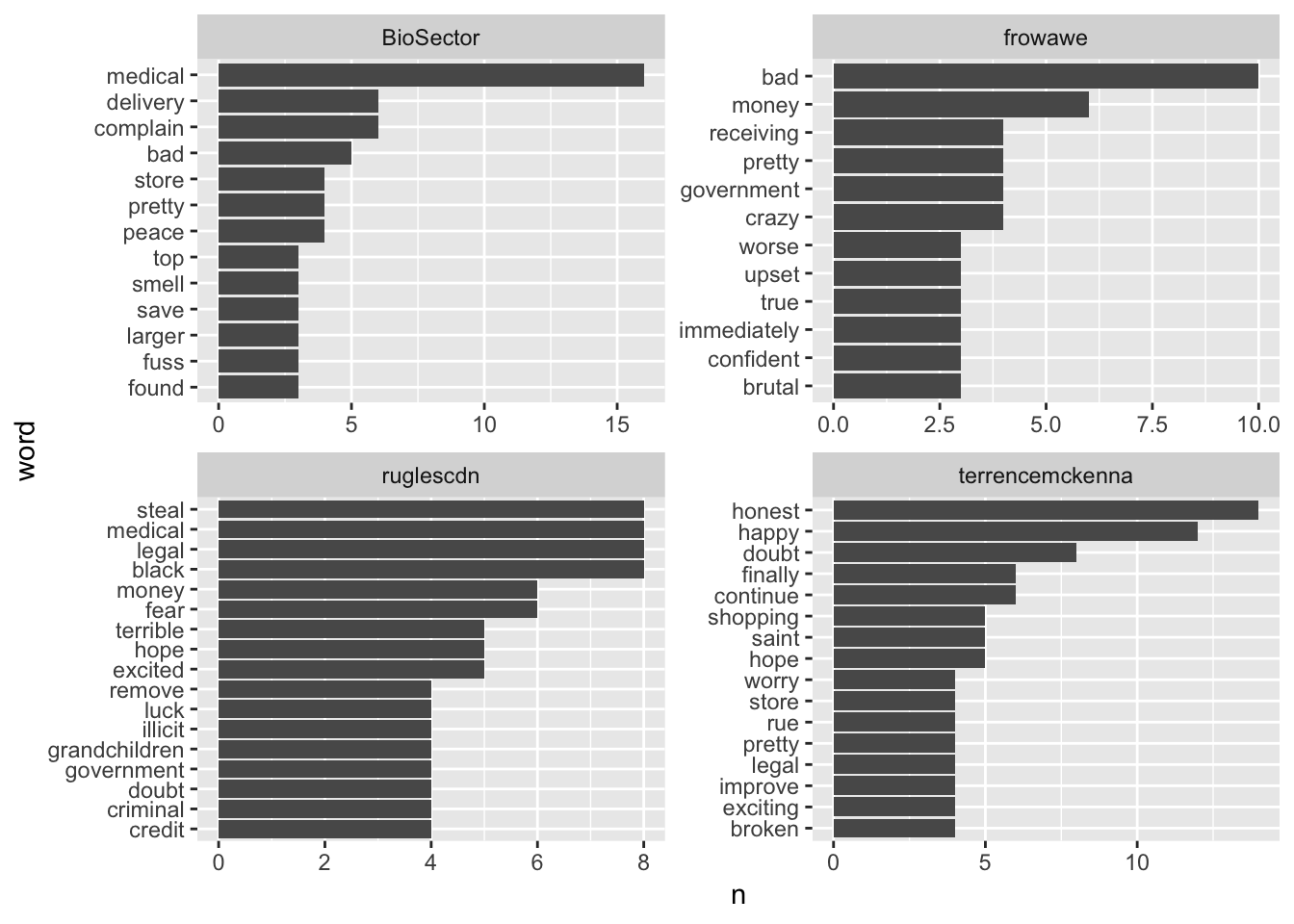

The output of the most frequently used words posted by individuals may be interesting. But to what extent is it insightful? One should know the specific sentiment these words annotate. The following chart displays counts of all the words from the previous scheme. Most importantly, these words are categorized within the sentiments from nrc lexicon.

data_sentiment %>%
    # Count by word and author
    group_by(word,author)%>%
    mutate(n=n())%>%
    # Group by author
    filter(author %in% c("BioSector", "ruglescdn",  "terrencemckenna", "frowawe" ))%>%
    group_by(author) %>%
    top_n(30) %>%
    ungroup() %>% 

    # Set up the plot with aes()
    ggplot(aes(word,n)) +
    geom_col(show.legend = FALSE) +
    facet_wrap(~ sentiment, scales = "free") +
    coord_flip()+
    ylab("Count")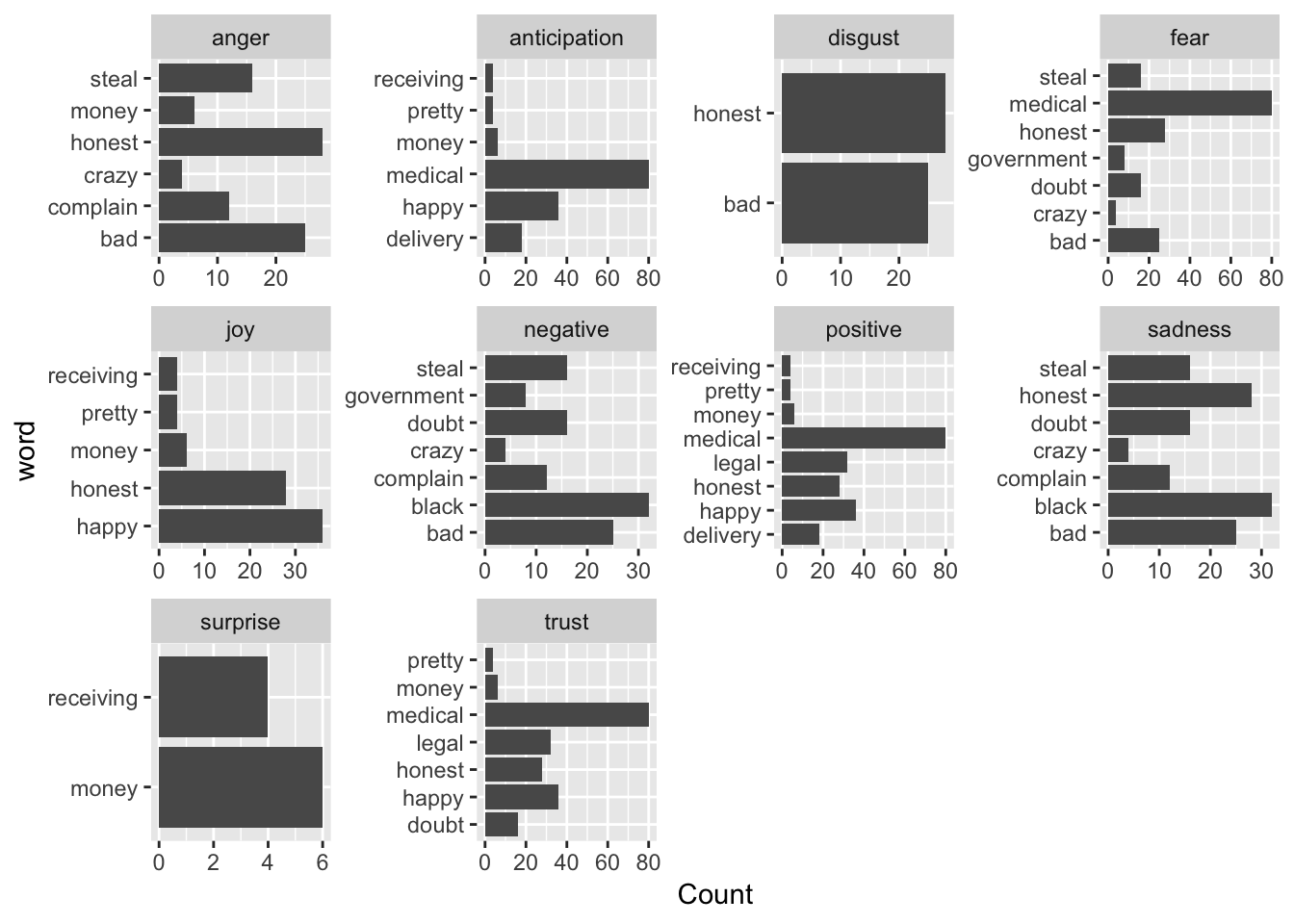

You can see that BioSector, ruglescdn, terrencemckenna, and frowawe express in a number of ways. Even though they do not express disgust or surprise too often, I could not determine what is their most common sentiment. Since a table is not as space demanding as any rigorous plot, the one mentioned below summarizes and counts sentiment related words by their authors.

data_sentiment %>%
    filter(author %in% c("BioSector", "ruglescdn",  "terrencemckenna", "frowawe" ))%>%
    group_by(sentiment) %>%
    summarise(count=n())%>%
    arrange(desc(count))

## # A tibble: 10 x 2
##    sentiment    count
##    <chr>        <int>
##  1 positive       122
##  2 trust           83
##  3 negative        77
##  4 anticipation    70
##  5 fear            45
##  6 sadness         35
##  7 anger           32
##  8 joy             30
##  9 surprise        26
## 10 disgust         20

Amazing! BioSector, ruglescdn, terrencemckenna, and frowawe create mostly positive sentiment!

My next goal was to allocate the most positive and negative authors. For this purpose, I created a new variable percent. count() groups author, sentiment, and author_total . Then, it creates a new variable n, and calls ungroup() afterwards. Consequently, n is nothing but the number of words by author within a particular sentiment.

# Which authors use the most negative words?
data_sentiment %>% 
    count(author, sentiment, author_total) %>%
    # Define a new column percent
    mutate(percent=n/author_total) %>%
    # Filter only for negative words
    filter(sentiment %in% c("negative","positive")) %>%
    # Arrange by percent
    arrange(desc(percent))%>%
    group_by(sentiment)%>%
    top_n(5) %>%
    ungroup()%>%
  
  ggplot(aes(author,percent)) +
    geom_col(show.legend = FALSE) +
    facet_wrap(~ sentiment, nrow = 2, scales = "free") +
    coord_flip()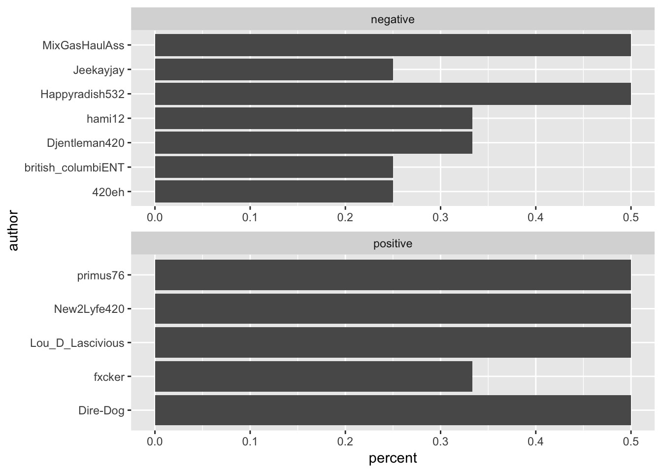

The plot above discloses the information of authors, responsible for the greater portion of positive and negative comments. There are two things worthy of mention: i.) the two sets do not intersect so these authors are not ambiguous. ii.) there appears to be “no author” from the group of most frequent contributors.

I also assumed that BioSector, ruglescdn, terrencemckenna, and frowawe are the most popular ones or at least have posted the most popular comments.

#the Most Popular Comments
dataset %>%
  select(id,author,likes)%>%
  arrange(desc(likes))%>%
  head(5)

##    id           author likes
## 1 436        [deleted]    20
## 2 444 captain_deadfoot    19
## 3 265   AgentChimendez    18
## 4 172        [deleted]    16
## 5 184          jamagut    15

To my surprise, no one appears in these two groups simultaneously.

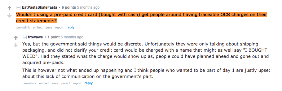
To have an idea about what drives the participants to like someone’s comment, one should read them! Below are a few screenshots of the top 3 ranked comments: SirWinnipegge complains about new prices in the local dispensary. Has he been buying weed on the black market for lower prices? If so, are the other cannabis users having the same experience? Then is legalizing marihuana an effective strategy to uproot black market cannabis trade? On the other hand, AgentChimendez celebrates the date: 10/17/2018 as the new milestone in Canadian history. He points out to the 20th of April, the World Cannabis Day, mostly referred to as 420. Lastly, captain_deadfoot’s comment was liked because he reacted to someone else outside of Canada. He emphasizes how friendly Canadian black market prices are in contrast to other countries. Again, it seems like the black market has already been supplying cannabis for a friendly price. Should the government introduce price ceiling to effectively compete with the black market?

#Least Popular Comments
dataset %>%
  select(id, author,likes) %>%
  arrange(likes) %>%
  head(5)

##    id         author likes
## 1 297       dubs2112   -10
## 2 351         Justos    -5
## 3  25     Hendrix194    -2
## 4  60      trekrlife    -2
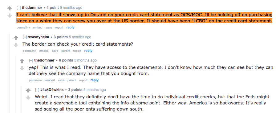
## 5 348 Happyradish532    -2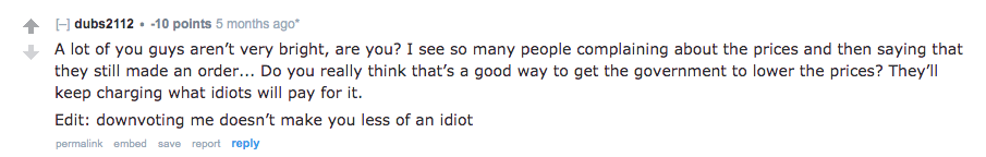

I particularly enjoyed dubs2112’s comments! He/she was constantly bullied (disliked) by others in the discussion because he/she basically calls people stupid for buying legal cannabis products.

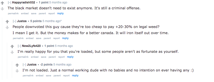The other posts with dislikes appear in the same thread. Happyradish532 and Justos celebrate the shock that the black market might incur. They seem comfortable with paying more for legal cannabis since it is supposed to weaken the black market.

Finally, let’s see how the sentiments - positive and negative - were developing during the first few weeks. This step was the most difficult one. First of all, I created a new data set sentiment_by_time from tidy_data. Since the time span for which the discussion was truly alive is really short, I rounded date to the unit of days and called the new variable date_floor. After grouping by date_floor, I created another new variable total_words, i.e. the number of total words per day. Again, I merged the data with nrc lexicon.

In the next step, I filtered the positive and negative sentiments in sentiment_by_time. Most importantly, I counted entries of the group: date_floor, sentiment, and total_words, and created new variable percent which is the ratio of counts per group and total words submitted in a day.

The purpose of this plot is to demonstrate the long-term development of positive vs. negative sentiment. Additionally, method = "lm" regresses percent on time and plots slopes of the development curves. Unfortunately, the time span in my model is very short and I do not yet mak any conlusions.

sentiment_by_time <- tidy_data %>%
    # Define a new column using floor_date()
    mutate(date_floor = floor_date(date, unit = "1 day")) %>%
    # Group by date_floor
    group_by(date_floor) %>%
    mutate(total_words = n()) %>%
    ungroup() %>%
    # Implement sentiment analysis using the NRC lexicon
    inner_join(get_sentiments("nrc"), by="word")

sentiment_by_time %>%
    # Filter for positive and negative words
    filter(sentiment %in% c("positive","negative")) %>%
    filter(date_floor < ymd("2018-11-10")) %>%
    # Count by date, sentiment, and total_words
    count(date_floor, sentiment, total_words) %>%
    ungroup() %>%
    mutate(percent = n / total_words) %>%
    
    # Set up the plot with aes()
    ggplot(aes(date_floor,percent,col=sentiment)) +
    geom_line(size = 1.5) +
    geom_smooth(method = "lm", se = FALSE, lty = 2) +
    expand_limits(y = 0)+
    ggtitle("Sentiment Over Time")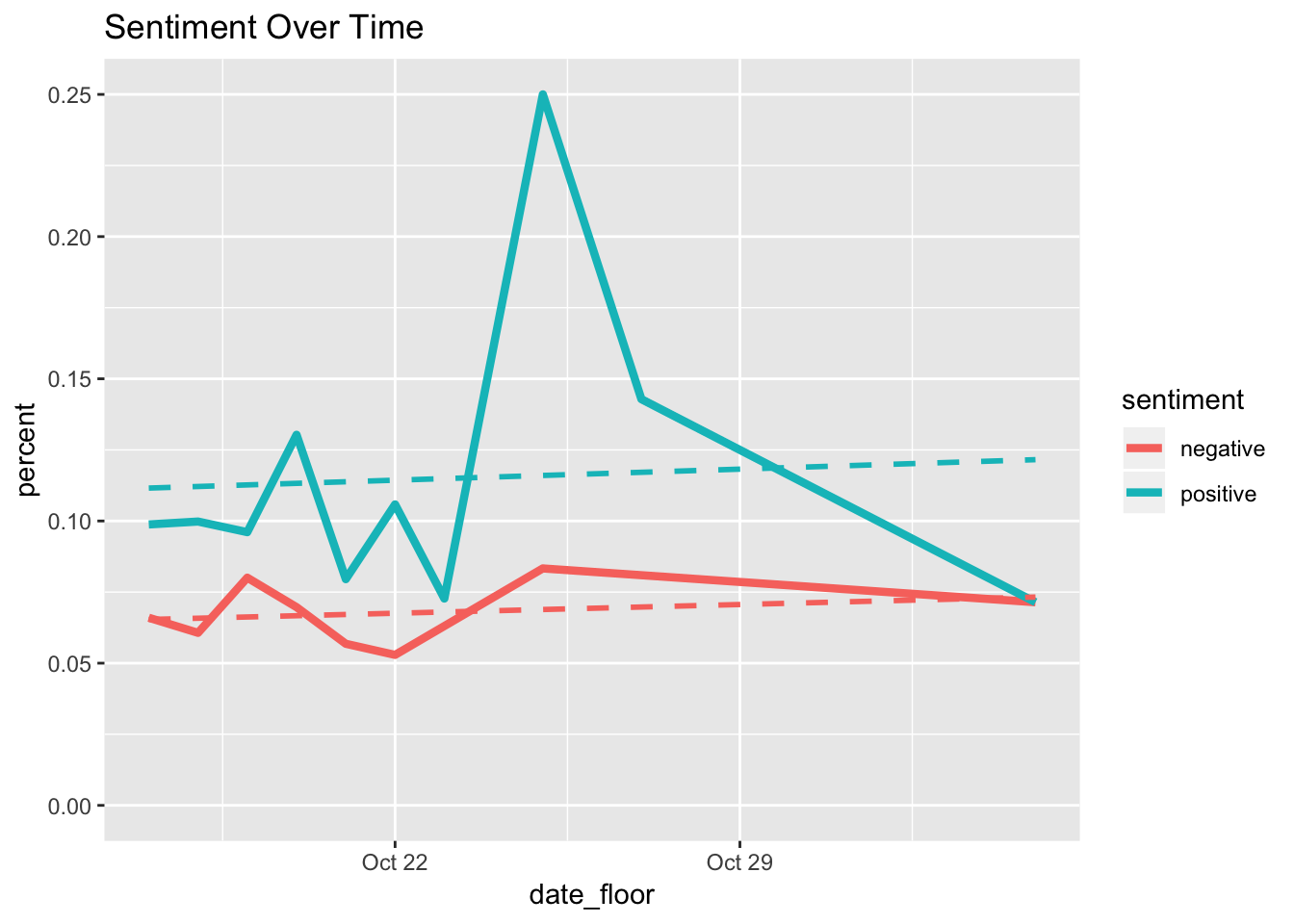

Nevertheless, it seems like positive and negative sentiments exhibit the same mild but positive slopes. Secondly, positive sentiment has much greater variation. Finally, both sentiments achieve their peaks shortly after October 22nd and decline later.

To see what stands behind the steep rise of positive sentiment, I found a few explanatory comments.

sentiment_by_time %>%
  filter(sentiment %in% c("positive","negative"))%>%
  filter( ymd("2018-10-22") < date_floor & date_floor < ymd("2018-10-29")) %>%
  group_by(date_floor, sentiment, total_words) %>%
  mutate(n=n()) %>%
  ungroup() %>%
  mutate(percent = n / total_words) %>%
  group_by(id)%>%
  mutate(max=max(percent)) %>%
  arrange(desc(max))

## # A tibble: 9 x 11
## # Groups:   id [5]
##   author likes date                   id word  date_floor         
##   <fct>  <int> <dttm>              <int> <chr> <dttm>             
## 1 Inter…     0 2018-10-25 04:40:29    13 ques… 2018-10-25 00:00:00
## 2 Inter…     0 2018-10-25 04:40:29    13 word  2018-10-25 00:00:00
## 3 Inter…     0 2018-10-25 04:40:29    13 legal 2018-10-25 00:00:00
## 4 Inter…     0 2018-10-25 04:40:29    13 ille… 2018-10-25 00:00:00
## 5 Diabl…     1 2018-10-27 23:24:02     6 child 2018-10-27 00:00:00
## 6 h3xad…     2 2018-10-23 04:59:38     7 legal 2018-10-23 00:00:00
## 7 h3xad…     2 2018-10-23 04:59:38     7 money 2018-10-23 00:00:00
## 8 Alypi…     0 2018-10-23 12:32:16    14 legal 2018-10-23 00:00:00
## 9 Hendr…     0 2018-10-23 00:01:04    20 eat   2018-10-23 00:00:00
## # … with 5 more variables: total_words <int>, sentiment <chr>, n <int>,
## #   percent <dbl>, max <dbl>

First of all, we can see that the positive sentiment achieved its peak on October 25th and was caused by a post written by IntermolecularButter (comment id 13). Another important observation is the fact that even though the time span was 1 week, there were only 7 new comments during that time! Less comments stand for less number words, therefore mutate(percent = n / total_words) may fluctuate a lot. Here, the peak is caused by the fact that the denominator was higher before October 22nd, resulting in a lower value of percent.

Nonetheless, let’s see what IntermolecularButter posted.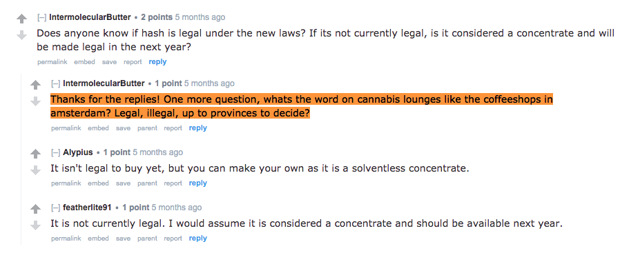

It is not very insightful, is it? The main reason why this post creates a positive sentiment, in addition to the explanation of high variation, is because the twelve words from the comment are associated with positive sentiment! Only one word - illegal - is considered negative. On top of that, sentiment was joined to the data set by inner_join(). By default, the result is that the data frame filtered words that were not present in the lexicon. For example, I noticed the word “thanks”" is not in nrc lexicon even though its connotation is definitely positive.

Conclusion

The analysis covered three topics; i.) web scraping using rvest package, ii.) cannabis legalization in Canada, and iii.) sentiment analysis. First of all, rvest provides enough flexibility to extract an HTML code from static web page and is therefore ideal for web scraping with R. However, I would suggest using API’s whenever possible to ease your job. Secondly, the discussion on cannabis legalization was not alive as one would expect. It seems that concerns about cannabis users’ privacy were not clearly communicated from the government as is evident from the comments. Additionally, during the time of this discussion posting, the consumers seem to be concerned about the price of legal cannabis being higher than the black market pricing. Lastly, sentiment analysis may not be a reliable approach when it comes to analyzing new policies, especially when something was decriminalized. One can see that more than legalization itself, the cannabis community was rather concerned about prices and privacy.